MATLAB使用指南

MATLAB(矩阵实验室)是MATrix LABoratory的缩写,是一款由美国The MathWorks公司出品的商业数学软件。MATLAB是一种用于算法开发、数据可视化、数据分析以及数值计算的高级技术计算语言和交互式环境。除了矩阵运算、绘制函数/数据图像等常用功能外,MATLAB还可以用来创建用户界面及与调用其它语言(包括C,C++,Java,Python和FORTRAN)编写的程序。本文主要介绍MATLAB中常用命令,方便规范使用。

MATLAB 的替代品:

  • Python是一门完全免费的通用编程语言,以开源的方式提供了大量各类用途的库与包,如 Numpy (数值计算)、 SciPy (数学、科学和工程计算)、 Matplotlib (类似MATLAB中plot的绘图工具)等等。
  • Octave是GNU项目成员之一,提供了与MATLAB语法兼容的开放源代码科学计算及数值分析的工具。
  • 对于航天器轨道计算、任务分析等,可以尝试General Mission Analysis Tool (GMAT)。GMAT提供了图像化界面或脚本两种接口,相比于STK,GMAT的深空探测相关功能更加强大,可配置的资源也更多。
  • GNU Radio是一个对学习,构建和部署软件定义无线电系统的免费软件工具包,可通过Python或类似于Simulink/Labview的图形化界面调用。 紫丁香、龙江等卫星的业余无线电接收解调软件就是在GNU Radio基础上开发并开源发布的。
  • Robot Operating System (ROS)是一种针对于满足不同机器人软件协同工作的灵活软件框架。目的在于提高软件模块化能力和复用能力,并实现不同任务间的数据/信号量的有效共享,方便多种机器人平台之间创建复杂和鲁棒的机器人行为,同时它也是一种工具库的约定与集合。

下载链接: https://www.iemblog.com/?s=matlab

I. 随机数

Matlab中的rand()函数产生的是伪随机数,但一般用来也可以接受。但是,如果我们知道伪随机数的初始状态,那么产生的伪随机数是唯一确定的。问题来了,Matlab每次启动会重置rand()和randn()的初始状态(重置为0),也就是说,你产生的随机数会出现两次随机数一模一样的情况。

1
2
3
4
5
6
7
8
9
10
11
12
13
14
15
16
17
18
19
20
21
22
23
24
25
>> rand('state',0)
>> rand(3,1)

ans =

0.9501
0.2311
0.6068

>> rand(3,1)

ans =

0.4860
0.8913
0.7621

>> rand('state',0)
>> rand(3,1)

ans =

0.9501
0.2311
0.6068

设定初始状态的好处是,只需要保存那时的初始状态再运行一遍程序你就可以重现之前的计算过程和结果。缺点是虽然程序使用了随机数,但由于(每次启动后)初始状态一样,实际运行出来却是相同的重复过程,你需要人工设定一个保证随机性的初始状态。

I.I. 设置初始状态

设置随机数初始状态有三种语法形式:

1
rand('seed', S)

S是表示初始状态的整数。seed、state、twister就比较奇怪,令人捉摸不透,不知道该选用哪个。这实际上是产生随机数的不同算法。seed表示采用v4版本的随机数产生器,state是v5版本的随机数产生器,最后的twister用的则是Mersenne Twister随机数产生器。前两个随机数产生器都是“flawed”,推荐大家使用twister随机数产生器。

新版的Matlab默认采用Mersenne Twister随机数产生器,rng(S) 函数表示设定初始状态,rng('shuffle') 表示随机分配一个初始状态。所以现在只需要记住rng()函数设置初始状态,然后用rand产生随机数就可以了。

1
2
rng(1);
A = rand(2,2)

I.II. 产生非重复的随机数

2012版本之后的用户比较方便,在产生随机数之前使用rng('shuffle')洗一下就可以(shuffle是洗牌的意思)。

以前推荐的是rand('state',sum(100*clock))来根据当前时间设定初始状态,但时间始终是递增的,而且变化幅度相对来说很小,效果不是很好。有很多人用别的方式设定初始状态(如rand('twister', fix(mod(1e11*(sum(clock)-2009), 2^31)));),为简便起见,个人推荐采用新版Matlab中rng函数语法,即

1
rand('twister',mod(floor(now*8640000),2^31-1));

II. 添加路径

1
2
3
4
5
6
7
8
% 添加绝对路径, 并未添加其子文件夹
addpath('D:\Workspace\Matlab\DL\DeepLearnToolbox-master');
% 添加绝对路径,其子文件夹进搜索路径
addpath(genpath('D:\Workspace\Matlab\DL\DeepLearnToolbox-master'));
% 移除绝对路径
rmpath('D:\Workspace\Matlab\DL\DeepLearnToolbox-master')
% 移除多个绝对路径
rmpath(genpath('D:\Workspace\Matlab\DL\DeepLearnToolbox-master'))

III. 数据集划分

划分数据集,产生训练集和测试集。

1
2
3
4
5
6
7
8
9
10
11
12
13
14
15
16
% Split training-testing data
rate = 0.5;
rand('seed',12345);
randn('seed',12345);
[n d] = size(X);
% random index
r = randperm(n);

% training samples
ntrain = round(rate*n);
Xtrain = X(r(1:ntrain),:);
Ytrain = Y(r(1:ntrain),:);

% test set
Xtest = X(r(ntrain+1:end),:);
Ytest = Y(r(ntrain+1:end),:);

IV. 矩阵除法求逆运算

如果要Moore-Penros广义逆的话可以用pinv(A); 如果只需要解方程Ax=b的一个解,可以直接x=A; 如果对精度要求比较高,不要用LU、QR,最好用SVD分解,根据需求来截断小奇异值。

inv:Y=inv(X)返回方阵X的逆矩阵,如果X病态或者高度奇异,则会显示警告信息。实际上,很少需要真的把矩阵的逆求出来,常见的使用失误主要出现在求解线性方程组AX=b。一种求解方法为x=inv(A)*b,但如要达到更快,更稳定,就得用X=A。这个算法使用高斯消去法,因此不产生逆矩阵。

如果A矩阵是非奇异方阵,则A,即inv(A)*B。而B/A是B乘A的逆矩阵,即B*inv(A)。具体计算时可不用逆矩阵而直接计算。使用符号“/”或“”会避免求逆,加速运算效率。换句话,(1/A)可以表示A的逆,这个算法使用高斯消去法,因此不产生逆矩阵。如果A矩阵不是方阵,可由以列为基准的Householder正交分解法分解,这种分解法可以解决在最小二乘法中的欠定方程或超定方程,结果是m×n的x矩阵。m是A矩阵的列数,n是B矩阵的列数。每个矩阵的列向量最多有k个非零元素,k 是A的有效秩。

“”:反斜线符号,矩阵左除。如果A是方阵,A(A)*B,只是他们的算法不一样。如果A是n*n的方阵,B是n*1的列向量,或n*?的矩阵,那么X=A=B的解。如果A很病态或者很奇异,很会显示警告信息。A(SIZE(A))计算A的逆,参见mldivide可得到更多信息。如果A是m*n的矩阵,m!=n,B是m*1或m*?的列向量,那么X=A=B(超定或者欠定)的最小二乘解。A的有效秩(effective rank)k有选主元的QR分解决定。Asolution X is computed that has at most k nonzero componentspercolumn。如果K<N,结果通常和pinv(A)*B不一样,后者是最小范数解。A(SIZE(A))用来求解A的广义逆。

mldivide(A,B):等价于A,A和B必须有一样多的行,除非A是个标量(这时就等于.)。如果A是个方阵,A(A)*B,只是两者算法不一样。如果A是m*n的矩阵,那么X=A=B(超定或欠定)的最小二乘解,即(AX-B)的范数极小。

奇异矩阵求逆用pinv。经查证,inv是matlab的built-in函数。而pinv则可以看到其源码,不长,其实就是调用另外一个built-in函数SVD进行奇异值分解,再截断奇异值进行求解而已。所以pinv实际上就是截断奇异值求逆。

1
2
3
4
5
假定拟计算一般矩阵A的Moore-Penrose广义逆A+,
1)对A做SVD:
A = U S V, 其中 U, V为酉方阵, S为一般对角阵;
2)将S非零元取逆, 零元不变, 然后专置得到一个一般对角阵T;
3)则广义逆为A+ = V* T U*, 其中 * 表示取矩阵的复共轭.

奇异矩阵如何处理:奇异矩阵求逆,给矩阵主对角线每一个元素加一个很小的量,如1e-6;强制可逆。

V. PLOT设置

Matlab画图(一):生成高质量的供发表和展示用的图
matlab绘图命令汇总

以下从一幅图可能涉及的多个方面进行罗列和演示:

1
2
3
4
5
6
7
8
9
10
11
12
13
14
15
16
17
18
19
20
21
22
23
24
25
26
27
28
29
30
31
32
33
34
35
36
37
38
39
40
41
42
43
44
45
46
47
48
49
50
51
52
53
54
55
56
57
58
59
60
61
62
63
64
65
66
67
68
69
70
71
72
73
74
75
76
77
78
79
80
81
82
83
84
85
86
87
88
89
90
91
92
93
94
95
96
97
98
99
100
101
102
103
104
105
106
107
108
109
110
111
112
113
114
115
116
117
118
119
120
121
122
123
124
125
126
127
128
129
130
131
132
133
134
135
136
137
138
139
140
141
142
143
144
145
146
147
148
149
150
151
152
close all

% 窗口初始最大化,推荐此命令
figure
set(gcf,'outerposition',get(0,'screensize'));
% 或者
set(gcf,'Position',get(0,'ScreenSize'))
% 或者
a=get(0);
figure('position',a.MonitorPositions);

% whitebg(1,'w') % 设置背景灰度

% 画图建议使用handle,方便命令调整

handle1=plot(a,'--pr','linewidth',1.5,'MarkerEdgeColor','r','MarkerFaceColor','m','MarkerSize',10)
% MarkerEdgeColor 标记点边框线条颜色颜色字符,如’g’, ’b’等
% MarkerFaceColor 标记点内部区域填充颜色颜色字符
% MarkerSize 标记点大小 数值,单位为points

% 或者使用RGB颜色,更多查看matlab绘图命令汇总
handle1=plot(x,y,'Color',[152 245 255]/256,'Linewidth',2);
handle1=plot(x,y,'Color','r','Linewidth',2);

hold on

% 有时候需要更改坐标轴刻度显示
set(gca, ’XTick’, [0 1 2]) % X坐标轴刻度数据点位置
set(gca,'XTickLabel',{'a','b','c'}) % X坐标轴刻度处显示的字符

% 待补充
set(gcf,'paperpositionmode','auto');

% 不采用
% 画图外观设置,type案例1,
set(gcf,'Position',[100 100 260 220]);
set(gca,'Position',[.13 .17 .80 .74]);
figure_FontSize=8;
set(get(gca,'XLabel'),'FontSize',figure_FontSize,'Vertical','top');
set(get(gca,'YLabel'),'FontSize',figure_FontSize,'Vertical','middle');
set(findobj('FontSize',10),'FontSize',figure_FontSize);
set(findobj(get(gca,'Children'),'LineWidth',0.5),'LineWidth',2);

% 采用
% 画图外观设置,type案例2。
% set(gca,'FontName','Times New Roman','FontSize',14) % 设置坐标轴刻度字体名称,大小
set(gca, 'fontsize', 14);
set(gca, 'XMinorTick', 'on');
set(gca, 'YMinorTick', 'on');
set(gca, 'XGrid', 'on');
set(gca, 'YGrid', 'on');
set(gca, 'LineWidth', 1.5);

% label设置
xlabel('Time (Second)', 'fontsize', 16);
ylabel('Amplitude', 'fontsize', 16);
ylabel('a','FontName','Times New Roman','FontSize',14,'Rotation',0)

% 坐标轴范围axis
ymin=**;
ymax=**;
xmin=**;
xmax=**;
% box = [-10.1 10.1 1.1*[min(t) max(t)]];
axis([xmin xmax ymin ymax]) % 设置坐标轴在指定的区间

% 同handle1命令
handle2=...
handle3=...

% legend说明
% LEGEND(string1,string2,string3, ...)
% LEGEND(...,'Location',LOC) 来指定图例标识框的位置

% 一个图例,可以直接放置
legend('First','Second','Third');
legend('First','Second','Third','Location','NorthEastOutside')
legend('First','Second','Third','Location','best') % 图例位置放在最佳位置

% 多个图例
handle_1=axes('position',get(gca,'position'),...
'visible','off');
handle_11=legend(handle_1,[handle_name handle_name handle_name handle_name handle_name],...
'legend_name',...
'legend_name',...
'legend_name',...
'legend_name',...
'legend_name');
handle_11.FontSize=6;
set(handle_11, 'Position', [0.45 0.8 0.1 0.1]); %位置属性,0-1设置

handle_2=axes('position',get(gca,'position'),...
'visible','off');
handle_21=legend(handle_2,[handle_name handle_name handle_name handle_name handle_name],...
'legend_name',...
'legend_name',...
'legend_name',...
'legend_name',...
'legend_name');
handle_21.FontSize=6; % 高版本使用
% set(handle_21,'fontsize',10) % 低版本使用
set(handle_21, 'Position', [0.6 0.8 0.1 0.1]); %位置属性,0-1设置

text(x,y,'Failure threshold','FontSize',16)
...

% title案例1
title('a','FontName','Times New Roman','FontWeight','Bold','FontSize',16)

% title案例2
string_1 = {'Predicting outcomes using SVR with linear kernel';
['Training Set: mse = ' num2str(error_1(2)) ' R^2 = ' num2str(error_1(3))];
['Testing Set mse = ' num2str(error_2(2)) ' R^2 = ' num2str(error_2(3))]};
title('标题Title','fontname','Times New Roman','Color','b','FontSize',20);

% title案例3
line1 = '适应度曲线MSE[ABCmethod]';
line2 = ['终止代数=', ...
num2str(iter-1),',种群数量NP=', ...
num2str(ABCOpts.ColonySize),')'];
line3 = ['Best c=',num2str(GlobalParams(1)),' g=',num2str(GlobalParams(2)), ...
' MSE=',num2str(GlobalMin)];
title({line1;line2;line3},'FontSize',20);


% 保存
% print函数原本不是用来进行图像保存了,而是操作打印机的,但是这里我们可以借用下
% print 可作为日常绘图的首选。对格式,分辨率等各项指标做非常细致的定义,适合直接出图。
% print(figure_handle,fileformat,filename)

print(gcf, '-depsc2', 'file_name.eps');
print('-depsc2','-r1000','file_name.eps');
% print('-dpsc','file_name.eps'); % 不采用,产生的图像在中间,tex中呈现漂浮在文字之上。
print(gcf, '-dpng', '-r280', 'file_name.png');
print(gcf,'-r300','-dpdf','file_name.pdf');
print(gcf,'-r300','-djpeg','file_name.jpeg');

% Matlab提供直接的saveas函数可以将指定figure中的图像或者simulink中的框图进行保存
% saveas可以保存matlab自认的fig格式的图像,用来最后细修很有意义。
% saveas(figure_handle,filename,fileformat)

saveas(gca,'file_name.eps','psc2')
% Matlab保存eps分成2个level,在使用saveas(gca,'**.eps')调用的level1的保存eps方式,所以彩色图像变成黑白的了。如果在命令中加入'psc2',此时,保存的图像是level2的,保存的图片就是eps格式的彩色图像。
saveas(gca,'file_name','png')
%saveas(gcf,file_name,'-r1000','epsc'); %错误

% 典型常用的带变量保存命令(推荐使用)
if save_figures
filenm = ['file_name_' num2str(variable_name)];
print('-depsc2','-r1000',['file_path',filenm]); %1000dpi,产生的图像在左下角,tex中正常显示。
saveas(gcf,['file_path',filenm], 'fig')
end

print()
用法:print(图形句柄,存储格式,文件名);
图形句柄,如果图形窗口标题栏是“Figure 3”,则句柄就是3.用gcf可以获取当前窗口句柄。
指定存储格式。常用的有:
png格式:'-dpng‘ (推荐这一种,与bmp格式一样清晰,文件也不大)
jpeg: ‘-djpeg‘(文件小,较清晰) tiff: ‘-dtiff‘
bmp: ‘-dbitmap‘(清晰,文件极大)
gif: ‘-dgif‘(文件小但不清晰)
文件名:自己给定
注意::print函数必须紧跟在plot函数之后使用。添加循环可以自动生成文件名。

V.I. 局部放大

利用 magnify.m 实现局部放大1

  1. magnify.m加载到 matlab 的安装路径中
  2. 运行程序,输出 figure
  3. 在 command window 中运行命令: magnify
  4. 在 figure 中编辑图形
    • 按ctrl键,拖动鼠标左键,(也可以不按ctrl键,拖动鼠标右键)就可以放大局部图像了
    • ctrl+左键固化,也可右键固化,‘<’和‘>’缩放方法范围(看细节-放大或者缩小细节)
    • ‘+’和‘-’缩放放大比例 (确定需要放大的区域 ‘+’ 选取更大的区域,‘-’号,选取小区域)
  5. 在 figure 中编辑图形,使用 标记‘2’处的图形‘edit’或者使用Tools > Edit plot,鼠标选中目标如图中标记‘1’处的框,或者外面的放大区域。 进一步可以执行目标删除、放缩+上下左右移动等
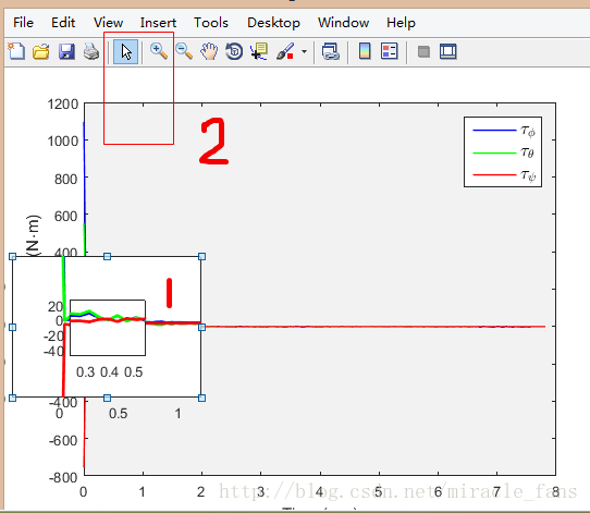
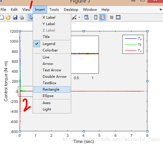
  6. 此时标记‘1’处的框已经被删除,上下左右调整放大框的位置,使用‘1’处的 insert 插入方框和箭头。
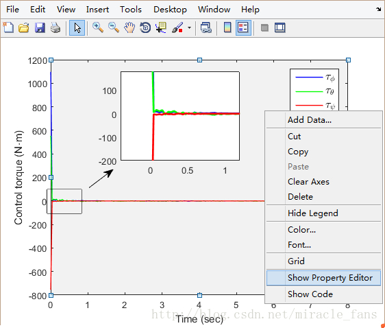
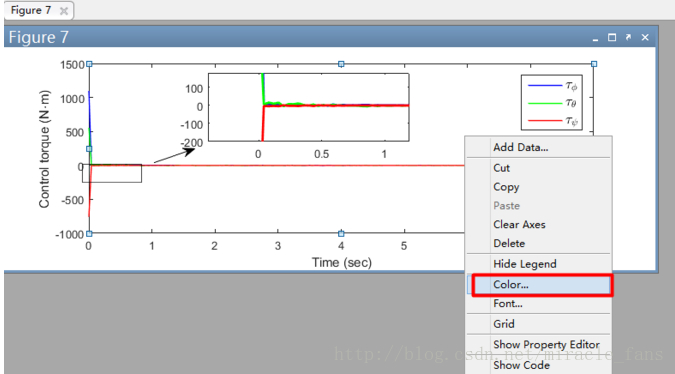
  7. 方框和箭头的位置,重回 edit 环境,在背景处右键-选择 show -property editor。选择‘white’在右面的三角号选择 ’ close ‘。或者如下图,使用背景-右键-color-white (方便快捷-推荐使用)。

VI. fill填充

对matlab中colormap的解释及fill、imshow的用法说明

VII. Legend控制

涉及到版本兼容问题,有些比较新的句柄属性在老版本Matlab中就用不起来,比如lineseries中的Annotation属性在我使用的R14SP1中就无法使用。

VII.I. Legend位置

LEGEND(...,'Location',LOC) 来指定图例标识框的位置

'North' 图例标识放在图顶端
'South' 图例标识放在图底端
'East' 图例标识放在图右方
'West' 图例标识放在图左方
'NorthEast' 图例标识放在图右上方(默认)
'NorthWest 图例标识放在图左上方
'SouthEast' 图例标识放在图右下角
'SouthWest' 图例标识放在图左下角
(以上几个都是将图例标识放在框图内)
'NorthOutside' 图例标识放在图框外侧上方
'SouthOutside' 图例标识放在图框外侧下方
'EastOutside' 图例标识放在图框外侧右方
'WestOutside' 图例标识放在图框外侧左方
'NorthEastOutside' 图例标识放在图框外侧右上方
'NorthWestOutside' 图例标识放在图框外侧左上方
'SouthEastOutside' 图例标识放在图框外侧右下方
'SouthWestOutside' 图例标识放在图框外侧左下方
(以上几个将图例标识放在框图外)
'Best' 图标标识放在图框内不与图冲突的最佳位置
'BestOutside' 图标标识放在图框外使用最小空间的最佳位置

利用位置属性进行精确设置

1
2
gca=legend( 'sinx', 4 );   
set( gca, 'Position', [0.1,0.1,0.9,0.9] );

[0.1,0.1,0.9,0.9] 分别为axes在figure中的左边界,下边界,宽度,高度,最小为0,最大为1(左边界,下边界为0,上边界,右边界为1)

1
2
3
4
5
figure
set (gca,'position',[0.1,0.1,0.9,0.9] );
x=1:0.1:10;
y=sin(x);
plot(x,y)

VII.II. 图例说明m条 (m < n)

如果一个图中我们画了n条曲线,但是我们只想加图例说明(legend)的只有m条 (m < n)。例如你有25条曲线,想显示其中1,6,11,16,21的legend,则

VII.II.I. Annotation命令

1
2
3
4
5
6
7
8
9
10
11
12
13
14
15
x = -3.14:0.1:3.14;
y1 = sin(x);
y2 = cos(x);
y3 = .1*exp(x);
y4 = y1.*y3;
hold on
h1 = plot(x, y1, 'r');
h2 = plot(x, y2, 'g');
h3 = plot(x, y3, 'k');
h4 = plot(x, y4, 'm');
hold off
xlim auto
set(get(get(h2, 'Annotation'), 'LegendInformation'), 'IconDisplayStyle', 'off');
set(get(get(h4, 'Annotation'), 'LegendInformation'), 'IconDisplayStyle', 'off');
legend('sin', 'exp');

EG.

1
2
3
4
for i = [2:5 7:10 12:15 17:20 22:25]
set(get(get(H(i),'Annotation'),'LegendInformation'),'IconDisplayStyle','off');
end
legend('1','6','11','16','21');

VII.III. legend命令

把想要标注的图形命令给个变量名,然后再legend命令中指定。

1
2
3
4
5
6
7
8
9
10
11
12
13
14
15
16
17
18
19
20
21
x = -3.14:0.1:3.14;
y1 = sin(x);
y2 = cos(x);
y3 = .1*exp(x);
y4 = y1.*y3;
hold on
h1 = plot(x, y1, 'r');
h2 = plot(x, y2, 'g');
h3 = plot(x, y3, 'k');
h4 = plot(x, y4, 'm');
THETA=linspace(0,2*pi,1000);
RHO=ones(1,1000)*2;
[X,Y] = pol2cart(THETA,RHO);
X=X+10;
Y=Y+10;
h5=plot(X,Y,'r--');

axis square;
hold off
xlim auto
legend([h1,h3,h5],'sin', 'exp','circle');

EG.

1
2
H = plot(data);
legend(H([1 6 11 16 21],'1,'6','11’,'16','21');

VII.IV. 多列legend

1
2
3
4
5
6
7
8
9
10
11
12
13
14
15
16
17
18
19
20
21
22
23
24
25
26
27
28
29
30
t=0:pi/100:2*pi;
y1=sin(t);
y2=cos(t);
y3=y1.*y2;
y4=0.5*(y1+y2);
hold on
h1=plot(t,y1,'-r')
%h11 = plot(t(1:10:end),y1(1:10:end),'o','MarkerFaceColor','r','MarkerEdgeColor','r');
h11 = plot(t(1:20:end),y1(1:20:end),'ro');
h2=plot(t,y2,'b-');
%h22 = plot(t(1:10:end),y2(1:10:end),'^','MarkerFaceColor','b','MarkerEdgeColor','b');
h22 = plot(t(1:20:end),y2(1:20:end),'b^')
h3=plot(t,y3,'c');
h4=plot(t,y4,'g');
hold off
[legh,objh,outh,outm]=legend([h1,h2],'y1','y2',1);
legend boxoff

% matlab 6.5.1
%set(objh(3),'marker','*');
%set(objh(5),'marker','.');

% matlab7
set(objh(4),'marker','o');
set(objh(6),'marker','^');


legh2=copyobj(legh,gcf);
[legh2,objh2]=legend([h3,h4],'y3','y4',2);
legend boxoff

只有第二个legend可拖动,而第一个legend不可拖动,原因不明。

VII.V. 避免legend覆盖曲线

给出的legend经常覆盖了某些曲线,这样就需要把legend分成几个,相对独立,这样可以使用鼠标随意移动,确保不遮挡曲线。

1
2
3
4
5
6
7
8
9
10
11
12
a=linspace(0,2*pi,100);
y1=100*sin(a);
y2=50*cos(a);
y3=tan(a);
y4=log(a);
y=[y1;y2;y3;y4];
figure
p=plot(a,y)
legend(p(1:2),'sin','cos');
ah=axes('position',get(gca,'position'),...
'visible','off');
legend(ah,p(3:4),'tan','log','location','west');

VII.VI. legend横排

1
2
hl = legend(H([1 6 11 16 21],'1,'6','11’,'16','21');
set(hl,'Orientation','horizon')

VII.VII. legend不显示方框

1
2
hl = legend(H([1 6 11 16 21],'1,'6','11’,'16','21');
set(hl,'Box','off');

VIII. errorbar

1
2
ERRORBAR(X,Y,L,U),X是自变量,Y是因变量,L是Y的变动下限,U是Y的变动上限
errorbar(X,Y,E) X是自变量,Y是因变量,E是Y的变动绝对差值。

IX. 柱状图

IX.I. 带有误差线(误差标记)的柱状图 errorbar

1
2
3
4
5
6
7
8
9
10
11
12
13
14
15
16
17
18
19
20
21
22
23
24
25
% 生成示例数据
x=1:10;
y=cumsum(randn(1,10));
lower = y - (rand(1,10));
upper = y + (rand(1,10));

% 由于errorbar函数使用相对差值在图形上绘图,所以
% 需要将绝对差值转变为相对差值。
L = y - lower;
U = upper -y;

% 绘图时需要设定 hold on
% 柱状图
clf;
figure(1);
hold on;
bar(x,y);
% 此处需要隐藏折线
errorbar(x,y,L,U,'Marker','none','LineStyle','none');

% 折线图
figure(2);
hold('on');
plot( x, y);
errorbar( x, y, L, U);

IX.II. 直方图的绘制

1
2
3
4
5
6
7
8
9
10
11
12
13
14
15
16
17
18
19
20
21
22
23
%% 直方图图的绘制
%直方图有两种图型:垂直直方图和水平直方图。而每种图型又有两种表现模式:累计式:分组式。
figure;
z=[3,5,2,4,1;3,4,5,2,1;5,4,3,2,5]; % 各因素的相对贡献份额
colormap(cool);% 控制图的用色
subplot(2,3,1);
bar(z);%二维分组式直方图,默认的为'group'
title('2D default');
subplot(2,3,2);
bar3(z);%三维的分组式直方图
title('3D default');
subplot(2,3,3);
barh(z,1);%分组式水平直方图,宽度设置为1
title('vert width=1');
subplot(2,3,4);
bar(z,'stack');%累计式直方图,例如:1,1+2,1+2+3构成了第一个bar
title('stack')
subplot(2,3,5);
bar3h(z,0.5,'stacked');%三维累计式水平直方图
title('vert width=1 stack');
subplot(2,3,6);
bar3(z,0.8,'grouped');%对相关数据的颜色进行分组,默认的位'group'
title('width=0.8 grouped');

IX.III. 柱状图的进阶

1
2
3
4
5
6
7
8
9
10
11
12
13
14
15
16
17
18
19
20
21
22
23
24
25
26
27
28
%% =========柱状图的进阶==========
figure;
y=[300 311;390 425; 312 321; 250 185; 550 535; 420 432; 410 520;];
subplot(1,3,1);
b=bar(y);
grid on;
set(gca,'XTickLabel',{'0','1','2','3','4','5','6'})
legend('算法1','算法2');
xlabel('x axis');
ylabel('y axis');
%使仅有的一组柱状图呈现不同颜色,默认的位相同颜色
data = [1.0, 1.0, 0.565, 0.508, 0.481, 0.745];
subplot(1,3,2);
b = bar(data);
ch = get(b,'children');
set(ch,'FaceVertexCData',[4;2;3;1;5;6]);%使用Indexed形式指定每组bar的颜色
set(gca,'XTickLabel',{'C0','C1','C2','C3','C4','C5'})
axis([0 7 0.0 1.0]);
ylabel('micro F-measure');
%使每个bar颜色不同,默认的是每个元素在不同组的颜色相同
data = [3, 7, 5, 2;4, 3, 2, 9;6, 6, 1, 4];
subplot(1,3,3);
b = bar(data);
ch = get(b,'children');
set(ch{1},'FaceVertexCData',[1;2;3]);%设置第一个元素在不同组的颜色
set(ch{2},'FaceVertexCData',[1;2;3]);%设置第二个元素在不同组的颜色
set(ch{3},'FaceVertexCData',[1;2;3]);
set(ch{4},'FaceVertexCData',[1;2;3]);

IX.IV. 彩色柱状图

1
2
3
4
5
6
7
8
9
10
11
12
13
14
15
16
17
18
19
20
21
22
23
24
25
26
27
28
29
30
31
32
33
34
35
36
37
38
39
40
41
42
43
44
45
46
47
48
49
50
51
52
%% 彩色柱状图
%用到的数据
n = 8;
Z = rand(n,1);
figure;
%默认图片
subplot(1,3,1);
bar(Z);
%简单的作图
% 这个图根据数据列中值的大小着色。每列中的值越大,颜色越突出
subplot(1,3,2);
h=bar(Z);
colormap(summer(n));
ch = get(h,'Children');
fvd = get(ch,'Faces');%针对矩阵时,只能用fvd=get(ch{col},'Faces'),下同
fvcd = get(ch,'FaceVertexCData');
[~, izs] = sortrows(Z,1);
for i = 1:n
row = izs(i);
fvcd(fvd(row,:)) = i;
end
set(ch,'FaceVertexCData',fvcd)
%图片会以渐变的方式着色,效果非常不错
subplot(1,3,3);
h=bar(Z);
ch = get(h,'Children');
fvd = get(ch,'Faces');
fvcd = get(ch,'FaceVertexCData');
[zs, izs] = sortrows(Z,1);
k = 128; % 准备生成128 *3 行的colormap
colormap(summer(k)); % 这样会产生一个128 * 3的矩阵,分别代表[R G B]的值
% 检视数据
whos ch fvd fvcd zs izs
% Name Size Bytes Class Attributes
%
% ch 1x1 8 double
% fvcd 66x1 528 double
% fvd 13x4 416 double
% izs 13x1 104 double
% zs 13x1 104 double
%
shading interp % Needed to graduate colors
for i = 1:n
color = floor(k*i/n); % 这里用取整函数获得color在colormap中行
row = izs(i); % Look up actual row # in data
fvcd(fvd(row,1)) = 1; % Color base vertices 1st index
fvcd(fvd(row,4)) = 1;
fvcd(fvd(row,2)) = color; % Assign top vertices color
fvcd(fvd(row,3)) = color;
end
set(ch,'FaceVertexCData', fvcd); % Apply the vertex coloring
set(ch,'EdgeColor','k');

IX.V. 绘制统计直方图

1
2
3
4
5
6
7
8
9
10
11
12
13
14
15
16
17
18
19
20
%% 绘制统计直方图
%hist(y):如果y是向量,则把其中元素放入10个条目中,且返回每条中的元素的个数;如果y为矩阵,则分别对每列进行处理,显示多组条形。
%[n,xout]=hist(y,x):非递减向量x的指定bin的中心。向量xout包含频率计数与条目的位置。
x=-10:.1:10;
y1=randn(2008,1);
y2=randn(2008,3);
figure;
colormap(winter);
subplot(2,2,1);
hist(y1);%把其中元素放入10个条目中
title('y1为向量,default,n=10');
subplot(2,2,2);
hist(y2);%分别对每列进行处理,显示多组条形
title('y2为矩阵');
subplot(2,2,3);
hist(y1,x);%用户也可以使用[n,xout]=hist(y1,x);bar(xout,n)绘制条形直方图
title('向量x指定条目');
subplot(2,2,4);
hist(y2,1000);%第二个参数为标量时指定bin的数目
title('nbins=1000');

IX.VI. 均值方差直方图

1
2
3
4
5
6
7
8
9
%% ========均值方差直方图========
a=[8 9 10 7 8 9];%mean
b=[1 1 1 1 1 1];%std
figure();
h=bar(a);
ch=get(h,'children');
set(ch,'FaceVertexCData',[4;2;3;1;5;6]);%使用Indexed形式指定每组bar的颜色
hold on;
errorbar(a,b,'k','LineStyle','none');

IX.VII. 散点图

1
2
3
4
5
6
7
8
9
10
11
12
13
14
15
16
17
18
19
20
21
22
23
24
%% =======散点图scatter , scatter3 , plotmatrix======
%scatter3(X,Y,Z,S,C):在由向量X、Y和Z指定的位置显示大小和颜色分别由S和C决定的离散点
figure;
[x,y,z] = sphere(16);
X = [x(:)*.5 x(:)*.75 x(:)];
Y = [y(:)*.5 y(:)*.75 y(:)];
Z = [z(:)*.5 z(:)*.75 z(:)];
S = repmat([10 2 5]*10,numel(x),1);
C = repmat([1 2 3],numel(x),1);
subplot(1,2,1);
scatter(X(:),Y(:),S(:),C(:));
title('scatter');
subplot(1,2,2);
scatter3(X(:),Y(:),Z(:),S(:),C(:),'filled'), view(-60,60);
title('scatter3');
%plotmatrix(X,Y)绘出X(p*M)与Y(p*N)的列组成的散度图(N,M)
figure;
X=randn(100,2);Y=randn(100,2);
subplot(1,3,1),plotmatrix(X);%等价于plotmatrix(X,X),除了对角上的图为X每一列的直方图hist(X(:,col))
title('plotmatrix(X)');
subplot(1,3,2),plotmatrix(X,X);
title('plotmatrix(X,X)');
subplot(1,3,3),plotmatrix(X,Y);
title('plotmatrix(X,Y)');

IX.VIII. 绘制区域图

1
2
3
4
5
6
7
8
9
10
11
%% =========绘制区域图===========
%区域图特点是:在图上绘制多条曲线时,每条曲线(除第一条外)都是把“前”条曲线作基线,再取值绘制而成。因此,该指令所画的图形,能醒目地反映各因素对最终结果的贡献份额。
figure;
x=1:2:9;% 注意:自变量要单调变化
y=magic(5);% 各因素的相对贡献份额,每一列相当于一个因素
colormap(spring);% 控制图的用色
area(x,y,4);%area(y)则以列下标作为自变量,第三个参数为基准线(默认为0)
set(gca,'layer','top');%图层设置为top层,显示网格
title('basevalue=4');
legend(' 因素 A',' 因素 B',' 因素 C','因素D','因素E');
grid on;

IX.IX. 绘制饼状图

1
2
3
4
5
6
7
8
9
10
%% =========绘制饼状图=========
%饼图指令pie和pie3用来表示各元素占总和的百分数。该指令第二个参数为与第一参数等长的 0-1
%向量,1使对应扇块突出。第三个参数指定个扇区的label
figure;
colormap(summer);% 控制图的用色
x=[16 17 21 25 21];
subplot(1,2,1);
pie(x,[0 0 0 0 1],{'0-10岁儿童','10-20岁儿童','20-35岁青年','35-55岁中年','55岁以上老年'});
subplot(1,2,2);
pie3(x,[0 0 0 0 1],{'0-10岁儿童','10-20岁儿童','20-35岁青年','35-55岁中年','55岁以上老年'});

IX.X. 绘制填色多边形

1
2
3
4
5
6
7
8
9
10
11
12
13
14
15
16
17
18
19
20
21
22
%% 绘制填色多边形。若每列的首尾元素不重合,则将默认把最后一点与第一点相连,强行使多边形封闭。
%fill和fill3用于绘制填色多边形
%fill(X1,Y1,C1,X2,Y2,C2,...)
%fill3(X1,Y1,Z1,C1,X2,Y2,Z2,C2,...)
%参数1和2为等长向量时,多边形的节点数由项链长度决定;而当其为矩阵时,每一列对应一个多边形
%参数3为颜色(用颜色字符r/g/b/c或[r g b]表示)
figure;
colormap(autumn);% 控制图的用色
n=10; % 多边形的边数
dt=2*pi/n;t=0:dt:2*pi;
t=[t,t(1)]; %fill 指令要求数据向量的首位重合,使图形封闭。
x=sin(t);y=cos(t);
subplot(1,2,1);
fill(x,y,[1 1 0]);axis off % 画填色多边形,隐去坐标轴。
X=[0.5 0.5 0.5 0.5;0.5 0.5 0.5 0.5;0 1 1 0];
Y=[0.5 0.5 0.5 0.5;0.5 0.5 0.5 0.5;0 0 1 1];
Z=[1 1 1 1;0 0 0 0;0 0 0 0];
C=[1 0 0 1;0 1 0 1;0 0 1 0];
subplot(1,2,2);
fill3(X,Y,Z,C);
view([-10 55]);
xlabel('x'),ylabel('y');box on;grid on;

IX.XI. 绘制离散数据杆状图

1
2
3
4
5
6
7
8
9
10
11
12
13
14
15
16
17
18
19
20
21
22
23
24
25
26
27
%% =======绘制离散数据杆状图===========
%stem和stem3函数用于绘制二维或三维的离散数据杆状图
%stem(Y)可以理解成绘制离散点的plot(y)函数
%stem(X,Y)可以理解成绘制离散点的plot(x,y)函数
%stem(...,'filled')改变数据点显示的空、实状态。
%stem(...,'LINESPEC')Linespec代表直线属性设置参量。
x=1:.1:10;
y=exp(x.*sin(x));
figure;
subplot(1,3,1);
plot(x,y,'.-r');
title('plot(x,y)');
subplot(1,3,2);
stem(x,y,'b');
subplot(1,3,3);
stem(x,y,':g','fill');
%绘制三维离散杆状图
th=(0:127)/128*2*pi;% 角度采样点
x=cos(th);
y=sin(th);
f=abs(fft(ones(10,1),128)); %对离散方波进行 FFT 变换,并取幅值
stem3(x,y,f','cd','fill');%绘制图形
view([-65 30]);
xlabel('Real'); %图形标注
ylabel('Imaginary');
zlabel('Amplitude');
title('FFT example');

IX.XII. 绘制方向和速度矢量图

1
2
3
4
5
6
7
8
9
10
11
12
13
14
15
16
17
18
19
20
21
22
23
24
25
26
27
28
29
30
31
32
33
34
35
36
37
38
39
40
41
42
43
44
45
46
%% =======绘制方向和速度矢量图=======
%compass-绘制罗盘图
%feather-绘制羽毛图
%quiver-绘制二维箭头图
%quiver3-绘制三维箭头图

%绘制罗盘图
figure;
wdir=[45 90 90 45 360 335 360 270 335 270 335 335];
knots=[6 6 8 6 3 9 6 8 9 10 14 12];
rdir=wdir*pi/180;
[x,y]=pol2cart(rdir,knots);% 极坐标转化为直角坐标
compass(x,y);
title('风向和风力')
%绘制羽毛图
figure;
alpha=90:-10:0;
r=ones(size(alpha));
m=alpha*pi/180;
n=r*10;
[u,v]=pol2cart(m,n);% 极坐标转化为直角坐标
feather(u,v);
title('羽毛图')
%罗盘图和羽毛图的比较
figure;
t=-pi/2:pi/12:pi/2; % 在 区间,每 取一点。
r=ones(size(t)); % 单位半径
[x,y]=pol2cart(t,r); % 极坐标转化为直角坐标
subplot(1,2,1),compass(x,y),title('Compass')
subplot(1,2,2),feather(x,y),title('Feather')
%绘制箭头图
figure;
[x,y] = meshgrid(-2:.2:2,-1:.15:1);
z = x .* exp(-x.^2 - y.^2);
[px,py] = gradient(z,.2,.15);
subplot(1,2,1);
contour(x,y,z), hold on
quiver(x,y,px,py), hold off, axis image
title('quiver示例');
[x,y,z]=peaks(15);
[nx,ny,nz]=surfnorm(x,y,z);%surfnorm求平面的法向量
subplot(1,2,2)
surf(x,y,z);
hold on;
quiver3(x,y,z,nx,ny,nz);
title('quiver3示例');

IX.XIII. 轮廓线图的绘制

1
2
3
4
5
6
7
8
9
10
11
12
13
14
15
16
17
18
19
20
21
22
23
24
%% ==========轮廓线图的绘制==========
%clabel-利用轮廓矩阵生成标签并在当前图形中显示
%contour-利用矩阵所给的值生成二维轮廓线
%contour3-利用矩阵所给的值生成三维轮廓线
%contourf-显示二维轮廓图并用色彩填充个轮廓线的间隙
%contourc-计算被其他轮廓函数占用的轮廓矩阵的低层函数
[x,y,z]=peaks;
n=15;% 等高线分级数
figure;
subplot(1,3,1);
h=contour(x,y,z,n);%绘制20条等高线
clabel(h);%当前图形中显示标签,标签前有'+'号且标签会根据轮廓线旋转,每条轮廓线仅有一个标签
title('simple contour,n=20');
subplot(1,3,2);
z=peaks;
[c,h]=contour(z,n);%绘制15条等高线
clabel(c,h);%标签前无'+'号,每天轮廓线可能有多个标签
title('调用clabel函数标注轮廓图')
subplot(1,3,3);
z=peaks;
[c,h]=contourf(z,n);
clabel(c,h,'FontSize',15,'Color','r','Rotation',0);%自定义标签
colorbar;
title('使用自定义标注并彩色填充轮廓线的间隙');

IX.XIV. Voronoi图和三角剖分

1
2
3
4
5
6
7
8
9
10
11
12
%% ========= Voronoi图和三角剖分========
%用Voronoi多边形勾画每个点的最近邻范围。Voronoi多边形在计算几何、模式识别中有重要应用。三角形顶点所在多边形的三条公共边是剖分三角形边的垂直平分线。
n=30;
A=rand(n,1)-0.5;
B=rand(n,1)-0.5; % 产生 30 个随机点
T=delaunay(A,B); % 求相邻三点组
T=[T T(:,1)]; %为使三点剖分三角形封闭而采取的措施
voronoi(A,B) % 画 Voronoi 图
hold on;axis square
fill(A(T(10,:)),B(T(10,:)),'y'); % 画一个剖分三角形
voronoi(A,B) % 重画 Voronoi 图,避免线被覆盖
title('Voronoi图和三角剖分');

IX.XV. 三角网线和三角曲面图

1
2
3
4
5
6
7
8
9
10
%% =========三角网线和三角曲面图========
figure;
X=6*pi*(rand(20,10)-0.5);Y=6*pi*(rand(20,10)-0.5);
R=sqrt(X.^2+Y.^2)+eps;Z=sin(R)./R;
tri=delaunay(X,Y); % 进行三角剖分
subplot(1,2,1),trimesh(tri,X,Y,Z);
title('三角网线');
subplot(1,2,2),trisurf(tri,X,Y,Z);
title('三角曲面图');
colormap(copper);brighten(0.5) % 增强亮度

IX.XVI. 彩带图ribbon

1
2
3
4
5
6
7
8
9
10
%% ============彩带图ribbon========
%ribbon(X,Y,WIDTH)和plot(X,Y)一样的,只不过每一列在三维中以分开的ribbon绘制
figure;
x=0:pi/100:2*pi;
x=repmat(x',1,10);
y=sin(x);
ribbon(x,y,0.4);% 画彩带图
% 至此彩带图已经生成。以下指令都是为了使图形效果更好、标识更清楚而用。
view([150,50]),shading interp,colormap(hot)% 设置视角、明暗、色图
light,lighting phong,box on % 设置光源、照射模式、坐标框

IX.XVII. 在特殊坐标系中绘制特殊图形

1
2
3
4
5
6
7
8
9
10
11
12
13
14
15
16
17
18
19
20
21
22
23
24
25
26
27
28
29
30
31
%% ==========在特殊坐标系中绘制特殊图形。=======
%利用polar函数在极坐标系中绘制图形
figure;
theta=0:.1:pi;
rho1=sin(theta);
rho2=cos(theta);
subplot(1,3,1);
polar(theta,rho1,'.-r');
hold on;
polar(theta,rho2,'--g');
title('极坐标系中绘图');
%另外一种和极坐标有关系的坐标系就是柱坐标系了
theta=0:pi/100:3*pi;
rho=sin(theta)+cos(theta);
[t,r]=meshgrid(theta,rho);
z=r.*t;
subplot(1,3,2);
[x,y,z]=pol2cart(t,r,z);%极坐标系向柱坐标系转化
mesh(x,y,z);%柱坐标系中进行绘图
title('柱坐标系中绘图');
view([-65 30]);
%将球坐标系转换为柱面坐标系
subplot(1,3,3);
delta=pi/100;
theta=0:delta:pi; % theta is zenith angle
phi=0:delta:pi; % phi is azimuth angle
[t p]=meshgrid(theta,phi);
r=ones(size(t));
[x,y,z]=sph2cart(t,p,r);%球坐标向柱坐标转化
mesh(x,y,z);%球坐标系中进行绘图
title('球坐标系中绘图');

IX.XVIII. 四维表现

1
2
3
4
5
6
7
8
9
10
11
12
13
14
15
16
17
18
19
20
21
22
23
24
25
26
27
28
%% ======四维表现========
%用色彩表现函数的特征
%当三维网线图、曲面图的第四个输入宗量取一些特殊矩阵时,色彩就能表现或加强函数的某特征,如梯度、曲率、方向导数等。
x=3*pi*(-1:1/15:1);y=x;[X,Y]=meshgrid(x,y);
R=sqrt(X.^2+Y.^2)+eps;Z=sin(R)./R;
[dzdx,dzdy]=gradient(Z);dzdr=sqrt(dzdx.^2+dzdy.^2); % 计算对 r 的全导数
dz2=del2(Z); % 计算曲率
figure;
subplot(1,2,1),surf(X,Y,Z),title('No. 1 surf(X,Y,Z)');
shading faceted,colorbar( 'horiz') ,brighten(0.2);
subplot(1,2,2),surf(X,Y,Z,R),title('No. 2 surf(X,Y,Z,R)');
shading faceted;colorbar( 'horiz');
%色彩分别表现函数的高度和半径特征
figure;
subplot(1,2,1),surf(X,Y,Z,dzdx) ;
shading faceted;brighten(0.1);colorbar( 'horiz');
title('No. 3 surf(X,Y,Z,dzdx)');
subplot(1,2,2),surf(X,Y,Z,dzdy);
shading faceted;colorbar( 'horiz');
title('No. 4 surf(X,Y,Z,dzdy)');
%色彩分别表现函数的 x 方向和 y 方向导数特征
figure;
subplot(1,2,1),surf(X,Y,Z,abs(dzdr)) ;
shading faceted;brighten(0.6);colorbar( 'horiz');
title('No. 5 surf(X,Y,Z,abs(dzdr))');
subplot(1,2,2),surf(X,Y,Z,abs(dz2));
shading faceted;colorbar( 'horiz');
title('No. 6 surf(X,Y,Z,abs(dz2))');

IX.XIX. 切片图和切片等位线图

1
2
3
4
5
6
7
8
9
10
11
12
13
14
15
16
17
18
19
20
%% ======切片图和切片等位线图=======
%利用 slice 和 contourslice 表现 MATLAB 提供的无限大水体中水下射流速度数据 flow 。 flow 是一组定义在三维空间上的函数数据。
%在本例中,从图中的色标尺可知,深红色表示“正速度”(向图的左方),深蓝表示“负速度”(向图的右方)。
% 以下指令用切面上的色彩表现射流速度
[X,Y,Z,V]=flow; % 取 4 个 的射流数据矩阵, V 是射流速度。
x1=min(min(min(X)));x2=max(max(max(X))); % 取 x 坐标上下限
y1=min(min(min(Y)));y2=max(max(max(Y))); % 取 y 坐标上下限
z1=min(min(min(Z)));z2=max(max(max(Z))); % 取 z 坐标上下限
sx=linspace(x1+1.2,x2,5); % 确定 5 个垂直 x 轴的切面坐标
sy=0; % 在 y=0 处,取垂直 y 轴的切面
sz=0; % 在 z=0 处,取垂直 z 轴的切面
figure;
slice(X,Y,Z,V,sx,sy,sz); % 画切片图
view([-12,30]);shading interp;colormap jet;axis off;colorbar;
% 以下指令用等位线表现射流速度
v1=min(min(min(V)));v2=max(max(max(V))); % 射流速度上下限
cv=linspace(v1,v2,15); % 在射流上下限之间取 15 条等位线
figure;
contourslice(X,Y,Z,V,sx,sy,sz,cv);view([-12,30]);
colormap jet;colorbar;box on;

IX.XX. 动态图形

1
2
3
4
5
6
7
8
9
10
11
12
13
14
15
16
17
18
19
20
21
22
23
24
25
%% =======动态图形=========
%简单二维示例-彗星状轨迹图
figure;
n=10;t=n*pi*(0:0.0005:1);x=sin(t);y=cos(t);
plot(x,y,'g');axis square;hold on
comet(x,y,0.01);hold off
%卫星返回地球的运动轨线示意
figure;
R0=1; % 以地球半径为一个单位
a=12*R0;b=9*R0;T0=2*pi; %T0 是轨道周期
T=5*T0;dt=pi/100;t=[0:dt:T]';
f=sqrt(a^2-b^2); % 地球与另一焦点的距离
th=12.5*pi/180; % 卫星轨道与 x-y 平面的倾角
E=exp(-t/20); % 轨道收缩率
x=E.*(a*cos(t)-f);y=E.*(b*cos(th)*sin(t));z=E.*(b*sin(th)*sin(t));
plot3(x,y,z,'g') % 画全程轨线
[X,Y,Z]=sphere(30);X=R0*X;Y=R0*Y;Z=R0*Z; % 获得单位球坐标
grid on,hold on,surf(X,Y,Z),shading interp % 画地球
x1=-18*R0;x2=6*R0;y1=-12*R0;y2=12*R0;z1=-6*R0;z2=6*R0;
axis([x1 x2 y1 y2 z1 z2]) % 确定坐标范围
view([117 37]),comet3(x,y,z,0.02),hold off % 设视角、画运动轨线
%色彩变幻‘在 256 色情况下,才可被正确执行.图片刷新可能会卡,单独执行spinmap可查看到效果
figure;
peaks;
spinmap;

IX.XXI. 影片动画

1
2
3
4
5
6
7
8
9
10
11
12
%% =======影片动画 =======
%三维图形的影片动画
figure;
shg,x=3*pi*(-1:0.05:1);y=x;[X,Y]=meshgrid(x,y);
R=sqrt(X.^2+Y.^2)+eps; Z=sin(R)./R;
h=surf(X,Y,Z);colormap(cool);axis off
n=12;mmm=moviein(n); %预设画面矩阵。新版完全可以取消此指令 。
for i=1:n
rotate(h,[0 0 1],25); %是图形绕 z 轴旋转 25 度 / 每次
mmm(:,i)=getframe; %捕获画面。新版改为 mmm(i)=getframe 。
end
movie(mmm,5,10) %以每秒10帧速度,重复播放5次

X. MATLAB数据导出origin画图

数据导出:

1
save afile.txt -ascii a

3D柱形图(3D Bars)的绘制使用Origin2017带误差棒的三维柱状图